1. Importing important price data
Every time I go to the supermarket, my wallet weeps a little. But how expensive is food around the world? In this notebook, we'll explore time series of food prices in Rwanda from the United Nations Humanitarian Data Exchange Global Food Price Database. Agriculture makes up over 30% of Rwanda's economy, and over 60% of its export earnings (CIA World Factbook), so the price of food is very important to the livelihood of many Rwandans.
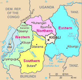
The map below shows the layout of Rwanda; it is split into five administrative regions. The central area around the Capital city, Kigali, is one region, and the others are North, East, South, and West.
In this notebook, we're going to import, manipulate, visualize and forecast Rwandan potato price data. We'll also wrap our analysis into functions to make it easy to analyze prices of other foods.
# Load the readr and dplyr packages
library('readr')
library('dplyr')

# Import the potatoes dataset
potato_prices <- read_csv("datasets/Potatoes (Irish).csv")

# Take a glimpse at the contents
glimpse(potato_prices)
2. Once more, with feeling
Many of the columns in the potato data aren't very useful for our analysis. For example, the adm1_name column is always "Rwanda", and cur_name is always "RWF". (This is short for Rwandan Franc; for context, 1000 RWF is a little over 1 USD.) Similarly, we don't really need any of the ID columns or the data source.
Even the columns we do need have slightly obscure names. For example, adm1_id isn't as clear as region, and mkt_name isn't as clear as market. One of the most types of data analysis disaster is to misunderstand what a variable means, so naming variable clearly is a useful way to avoid this. One trick is that any variable that includes a unit should include that unit in the variable name. Here, the prices are given in Rwandan Francs, so price_rwf is a good name.
# Import again, only reading specific columns
potato_prices <- read_csv("datasets/Potatoes (Irish).csv",
                         col_types = cols_only(adm1_name = col_character(),
                                               mkt_name = col_character(), cm_name = col_character(),
                                               mp_month = col_integer(), mp_year = col_integer(),
                                               mp_price = col_double()))

# Rename the columns to be more informative
potato_prices_renamed <- rename(potato_prices, region=adm1_name,
                                market=mkt_name, commodity_kg=cm_name,
                                month=mp_month, year=mp_year,
                                price_rwf=mp_price)

# Check the result
glimpse(potato_prices_renamed)
3. Spring cleaning
As is often the case in a data analysis, the data we are given isn't in quite the form we'd like it to be. For example, in the last task the month and year were given as integers. Since we'll be performing some time series analysis, it would be helpful if they were provided as dates. Before we can analyze the data, we need to spring clean it.
# Load lubridate
library('lubridate')

# Convert year and month to Date
potato_prices_cleaned <- mutate(potato_prices_renamed,
                               date = ymd(paste(year, month, "01")))
potato_prices_cleaned <- select(potato_prices_cleaned, -c(year, month))

# See the result
glimpse(potato_prices_cleaned)
4. Potatoes are not a balanced diet
As versatile as potatoes are, with their ability to be boiled, roasted, mashed, fried, or chipped, the people of Rwanda have more varied culinary tastes. That means you are going to have to look at some other food types!
If we want to do a similar task many times, we could just cut and paste our code and change bits here and there. This is a terrible idea, since changing code in one place doesn't keep it up to date in the other places, and we quickly end up with lots of bugs.
A better idea is to write a function. That way we avoid cut and paste errors and can have more readable code.
# Wrap this code into a function
read_price_data <- function(commodity){
    commodity_prices <- read_csv(
      paste("datasets/", commodity, ".csv", sep=""),
      col_types = cols_only(
        adm1_name = col_character(),
        mkt_name = col_character(),
        cm_name = col_character(),
        mp_month = col_integer(),
        mp_year = col_integer(),
        mp_price = col_double()
      )
    )

    commodity_prices_renamed <- commodity_prices %>%
      rename(
        region = adm1_name,
        market = mkt_name,
        commodity_kg = cm_name,
        month = mp_month,
        year = mp_year,
        price_rwf = mp_price
      )

    commodity_prices_cleaned <- commodity_prices_renamed %>%
      mutate(
        date = ymd(paste(year, month, "01"))
      ) %>%
      select(-month, -year)

}
# Test it
pea_prices <- read_price_data("Peas (fresh)")
glimpse(pea_prices)
5. Plotting the price of potatoes
A great first step in any data analysis is to look at the data. In this case, we have some prices, and we have some dates, so the obvious thing to do is to see how those prices change over time.
# Load ggplot2
library(ggplot2)

# Draw a line plot of price vs. date grouped by market
ggplot(potato_prices_cleaned, aes(x=date, y=price_rwf, group=market)) +
    geom_line(alpha=0.2) + ggtitle("Potato price over time")

6. What a lotta plots
There is a bit of a trend in the potato prices, with them increasing until 2013, after which they level off. More striking though is the seasonality: the prices are lowest around December and January, and have a peak around August. Some years also show a second peak around April or May.
Just as with the importing and cleaning code, if we want to make lots of similar plots, we need to wrap the plotting code into a function.
# Wrap this code into a function
plot_price_vs_time <- function(prices, commodity){
    prices %>%
      ggplot(aes(date, price_rwf, group = market)) +
      geom_line(alpha = 0.2) +
      ggtitle(paste(commodity, "price over time"))
    }

# Try the function on the pea data
plot_price_vs_time(pea_prices, "Pea")

7. Preparing to predict the future (part 1)
While it's useful to see how the prices have changed in the past, what's more exciting is to forecast how they will change in the future. Before we get to that, there are some data preparation steps that need to be performed.
The datasets for each commodity are very rich: rather than being a single time series, they consist of a time series for each market. The fancy way of analyzing these is to treat them as a single hierarchical time series. The easier way, that we'll try here, is to take the average price across markets at each time and analyze the resulting single time series.
Looking at the plots from the potato and pea datasets, we can see that occasionally there is a big spike in the price. That probably indicates a logistic problem where that food wasn't easily available at a particular market, or the buyer looked like a tourist and got ripped off. The consequence of these outliers is that it is a bad idea to use the mean price of each time point: instead, the median makes more sense since it is robust against outliers.
# Group by date, and calculate the median price
potato_prices_summarized <- potato_prices_cleaned %>% group_by(date) %>%
    summarize(median_price_rwf = median(price_rwf))

# See the result
glimpse(potato_prices_summarized)
8. Preparing to predict the future (part 2)
Time series analysis in R is at a crossroads. The best and most mature tools for analysis are based around a time series data type called ts, which predates the tidyverse by several decades. That means that we have to do one more data preparation step before we can start forecasting: we need to convert our summarized dataset into a ts object.
# Load magrittr
library(magrittr)

# Extract a time series
potato_time_series <- potato_prices_summarized %$% ts(median_price_rwf,
                        start=c(year(min(date)), month(min(date))),
                        end=c(year(max(date)), month(max(date))),
                        frequency=12
                        )

# See the result
plot(potato_time_series)

9. Another day, another function to write
Those data preparation steps were tricky! Wouldn't it be really nice if we never had to write them again? Well, if we wrap that code into a function, then we won't have to.
# Wrap this code into a function
create_price_time_series <- function(prices) {
    prices_summarized <- prices %>%
      group_by(date) %>%
      summarize(median_price_rwf = median(price_rwf))

prices_time_series <- prices_summarized %$%
  ts(
    median_price_rwf,
    start = c(year(min(date)), month(min(date))),
    end   = c(year(max(date)), month(max(date))),
    frequency = 12
  )
}

# Try the function on the pea data
pea_time_series <- create_price_time_series(pea_prices)
pea_time_series
10. The future of potato prices
All the preparation is done and we are ready to start forecasting. One question we might ask is "how do I know if I can trust our forecast?". Recall that both the potato and the pea data had strong seasonality (for example, potatoes were most expensive around August and cheapest around December). For agricultural data, a good forecast should show a similar shape throughout the seasons.
Now then, are we ready to see the future?
# Load forecast
library(forecast)

# Forecast the potato time series
potato_price_forecast <- forecast(potato_time_series)

# View it
potato_price_forecast

# Plot the forecast
autoplot(potato_price_forecast, main="Potato price forecast")

11. The final function
Nice! The forecast shows the spike in potato prices in late summer and the dip toward the end of the year.
With this analysis step, just as the previous steps, to make things repeatable, we need to wrap the code into a function.
# Wrap the code into a function
plot_price_forecast <- function(time_series, commodity){
    price_forecast <- forecast(time_series)
    autoplot(price_forecast, main = paste(commodity, " price forecast"))
}

# Try the function on the pea data
plot_price_forecast(pea_time_series, "Pea")

12. Do it all over again
That was a lot of effort writing all that code to analyze the potato data. Fortunately, since we wrapped all the code into functions, we can easily take a look at any other food type.
# Choose dry beans as the commodity
commodity <- "Beans (dry)"

# Read the price data
bean_prices <- read_price_data(commodity)

# Plot price vs. time
plot_price_vs_time(bean_prices, commodity)

# Create a price time series
bean_time_series <- create_price_time_series(bean_prices)

# Plot the price forecast
plot_price_forecast(bean_time_series)
